Top

Introduction

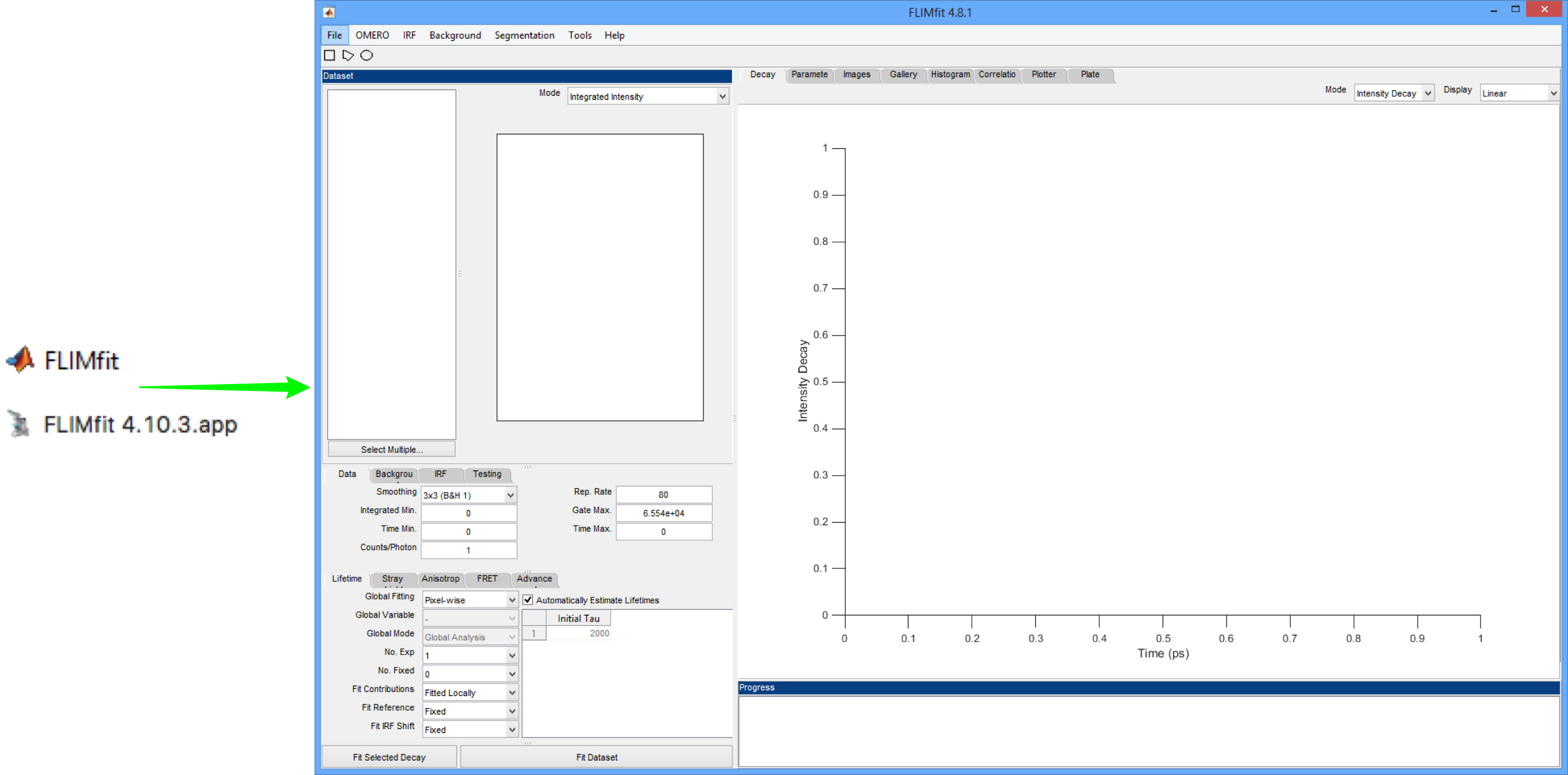
FLIMfit is a software tool that is designed to facilitate analysis and visualisation of time-resolved data from FLIM (Fluorescence Lifetime Imaging) measurements including time-correlated single photon counting (TCSPC) and wide-field time-gated imaging.

This is a tutorial-based workflow which describes the steps required to fit a bi-exponential model to the data from a single time-correlated single-photon counting (TCSPC) data file using the FLIMfit application when an Instrument Response Function (IRF) is available. It then explains how to perform a fit on a multi-file dataset.

The example files are Becker & Hickl GmbH .sdt files.

FLIMfit can connect to OMERO to load data directly from the OMERO server, or work with local files.

To use the data with OMERO, download a Zip archive of the the files: example-files.zip (47.4 MB).

Unzip the archive and import the following folders to the OMERO server, letting OMERO create new datasets from the folder, i.e. use default "New from Folder" for importing:

• IRF-in-file (contains the single data file and the corresponding IRF file)
• Multiple (contains the multiple data files and the corresponding IRF file)

Details on how to import data to OMERO are described in the Importing Data section.

A list of file formats supported by FLIMfit can be found on the OME website FLIMfit page.

Further details about FLIMfit can be found on the FLIMfit website.

Installing FLIMfit

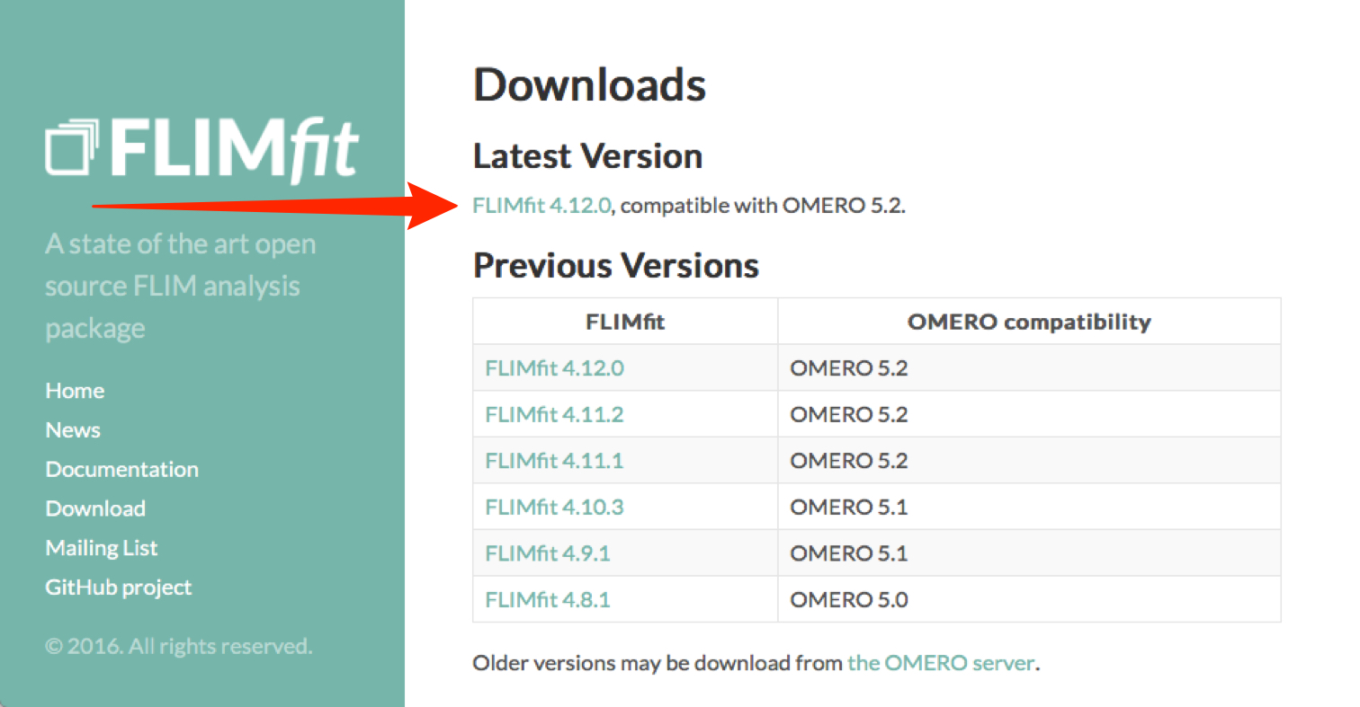
1. Use the link below to go to the FLIMfit downloads page.

   Click on the link under Latest Version to go to the downloads page for that version.

   http://flimfit.org/downloads/

   
   
   
   
   

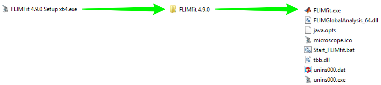
2. On Windows, the FLIMfit installer will automatically handle the MCR installation.

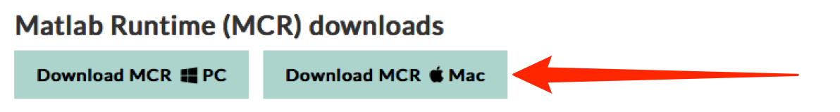
   Mac OS X users need to download and install the Matlab MCR from the downloads page for the FLIMfit version being used.

   This is required to ensure the correct version compatibility with FLIMfit.

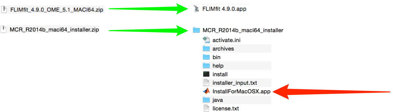
   Mac:

   
   
   

   

   
   

3. Expand the FLIMfit client archive and run the installer.

   
   

   Windows:

   

   Mac OS X:

   
   
   

Warning!

When running the Matlab MCR installer on Mac OS X the install wizard will give a message:

“On the target computer, append the following to your DYLD_LIBRARY_PATH environment variable:

/Applications/MATLAB/MATLAB_Compiler_Runtime/v84/runtime/maci64:/Applications/MATLAB/MATLAB_Compiler_Runtime/v84/sys/os/maci64:/Applications/MATLAB/MATLAB_Compiler_Runtime/v84/bin/maci64:”

Ignore this - the application will do it for you at run-time.

Using FLIMfit with OMERO

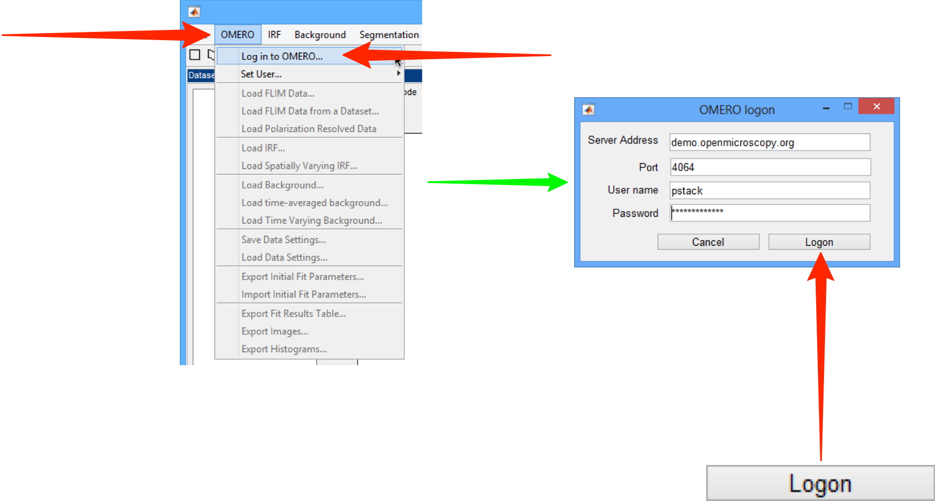
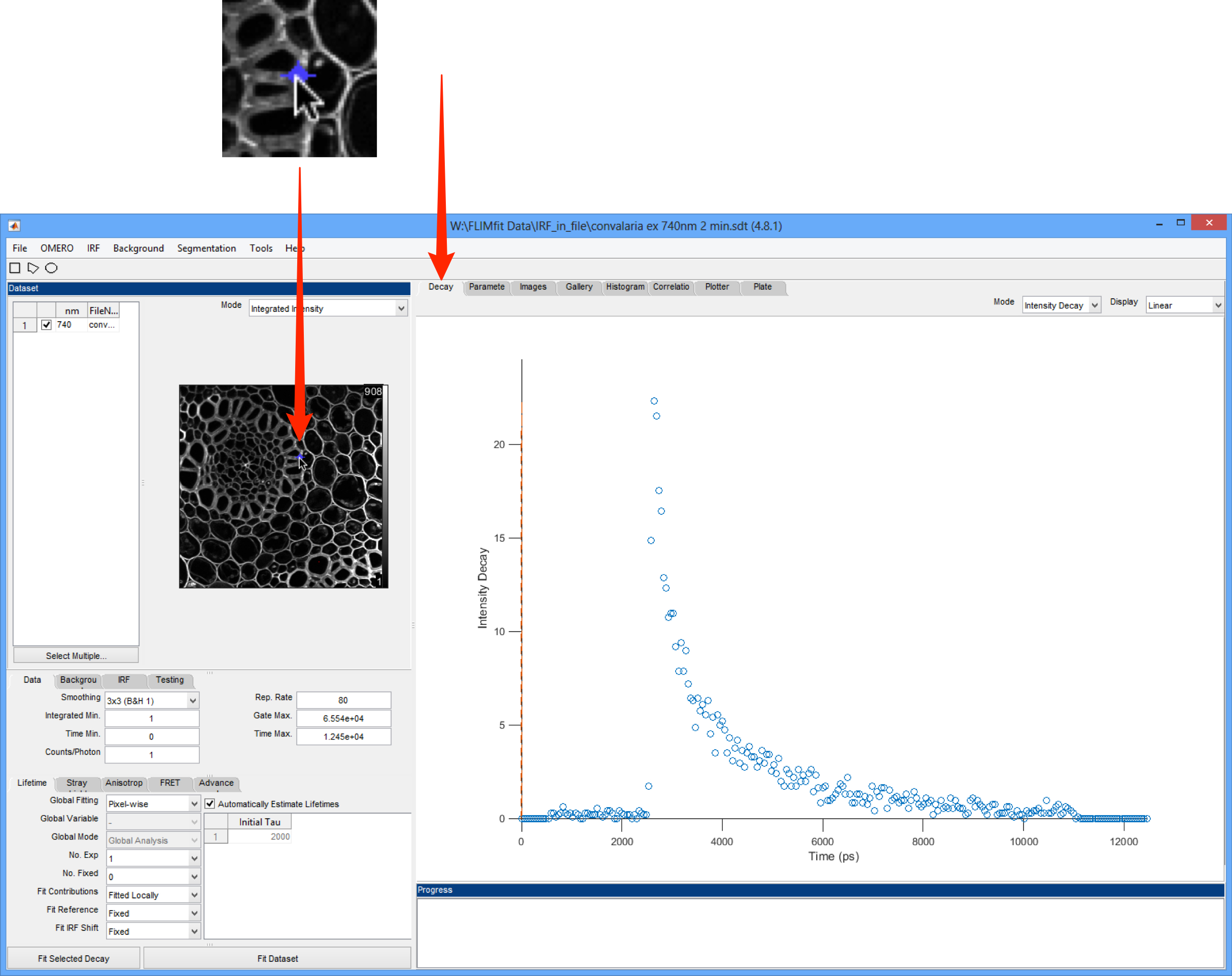
1. Open FLIMfit.

   
   
   
   
   

2. Click on the OMERO menu and select Log in to OMERO item.

   Enter the OMERO server address, port number, user name and password.

   Click Logon.

   
   
   
   
   








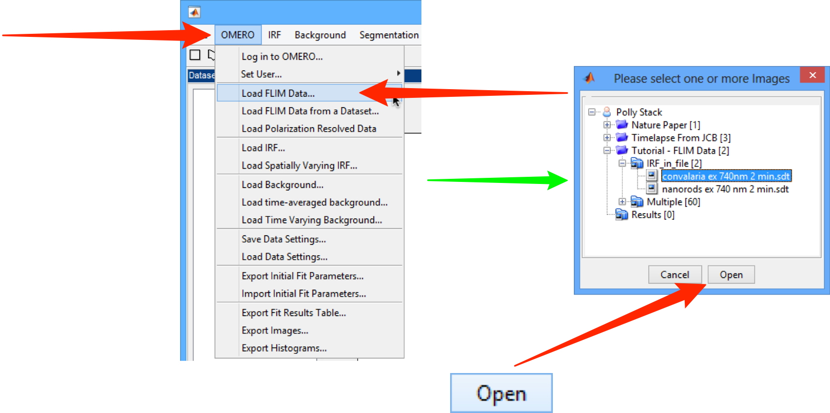
3. Click on the OMERO menu and select Load FLIM data.

   The OMERO data tree will be displayed in a pop-up window.

   Select the file:       convalaria ex 740nm 2 min.sdt

   Click Open.

   
   
   
   
   

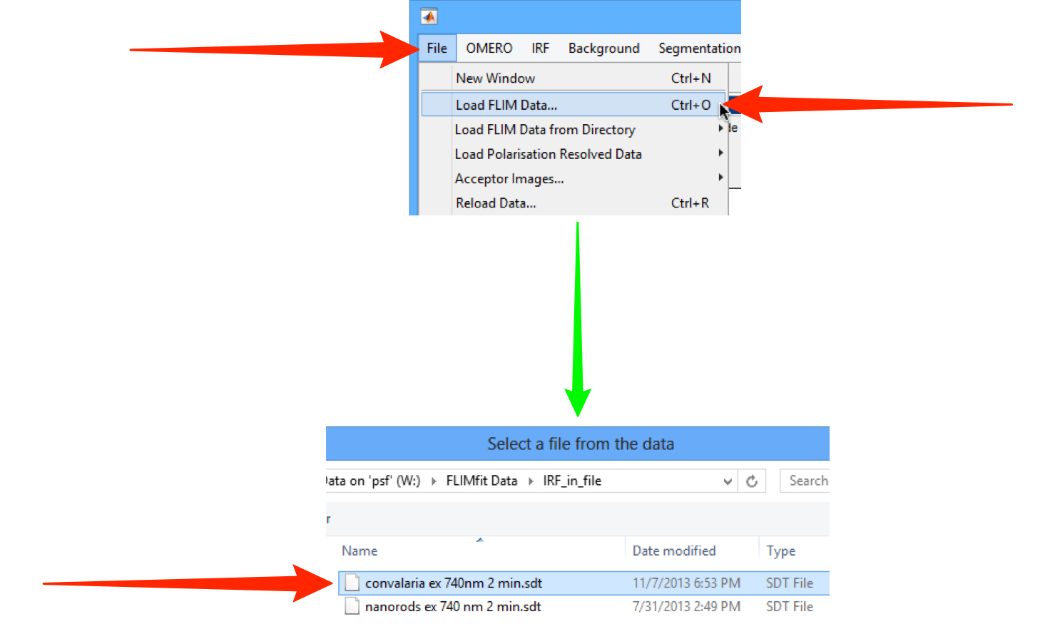
Loading data from disk

1. If loading a file from disk, click on the File menu and select Load FLIM Data....

   Select the file:        convalaria ex 740nm 2 min.sdt

   
   
   
   
   

Fitting data - single image

1. A greyscale intensity image of a pollen grain is visible in the upper part of the left-hand pane.

   Click on any pixel.

   The Decay tab to the right should be selected by default.

   A plot of the time-resolved data in that pixel can be seen.

   Choose a relatively bright region of the image to see a good example of a plot.

   
   
   
   
   



Note

A brief aside on Instrument Response Function (IRF)

In order to fit a model, FLIMfit requires some information about the system on which the data was acquired. It can get this information from what is referred to as an IRF - the system’s response to a known input.

In this example the IRF is read from a second .sdt file acquired on the same system, on the same day, as the pollen grain image. This is an image of a sample of gold nanorods. These have the convenient property of re-emitting the laser excitation pulse across a wide range of wavelengths. They therefore provide a pulse of light, of known (very short) duration, at the correct wavelength to pass into the detection channel.









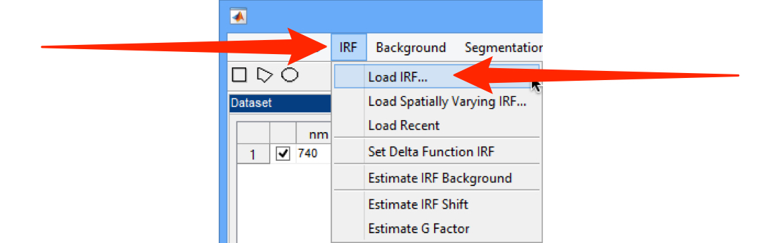
2. Click the OMERO menu and select Load IRF to load the IRF image from OMERO.

   In the left-hand pane, select the file:        nanorods ex 740 nm 2 min.sdt

   
   
   
   
   

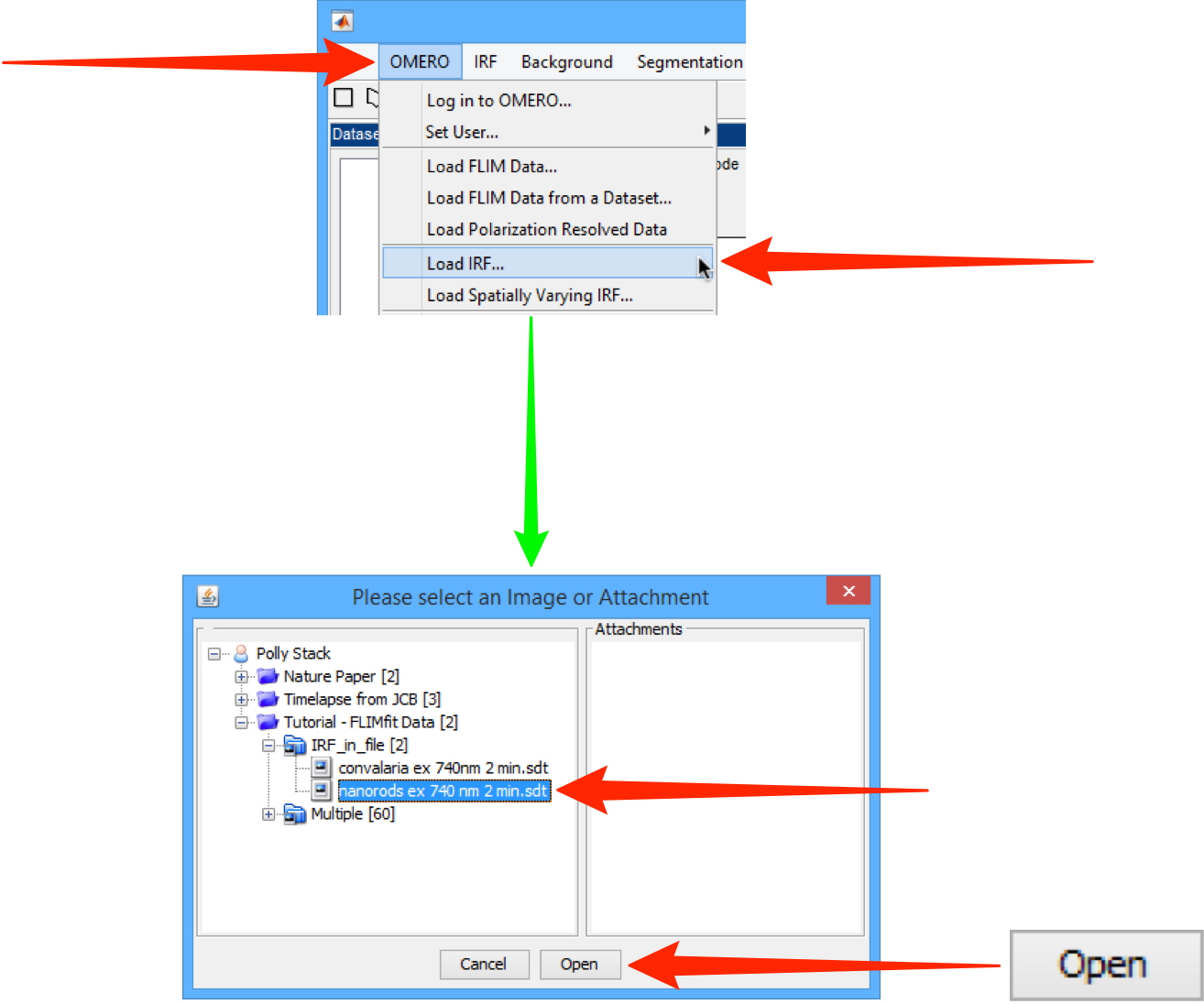
3. To load the IRF image from disk click the IRF menu and select Load IRF....

   Select the file:        nanorods ex 740 nm 2 min.sdt

   
   
   
   
   






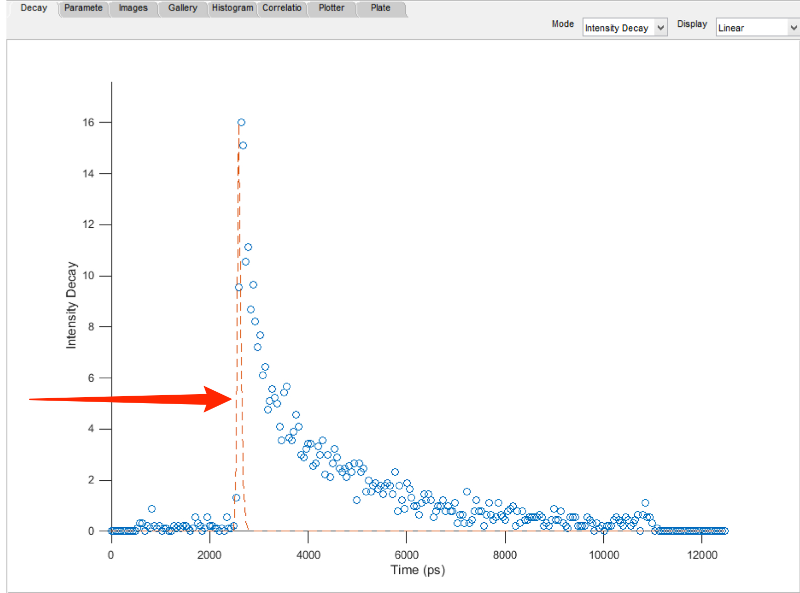
4. The IRF data will be superimposed as a red line on the plot in the Decay tab.

   
   
   
   
   
   
   

5. Set the Integrated Min to 90 to exclude the dark areas of the image.

   This colours the areas below the threshold red.

   Click Fit Selected Decay.

   A broken blue line appears in the fitted model.

   Normalised Residuals are displayed below data.

   
   
   
   
   






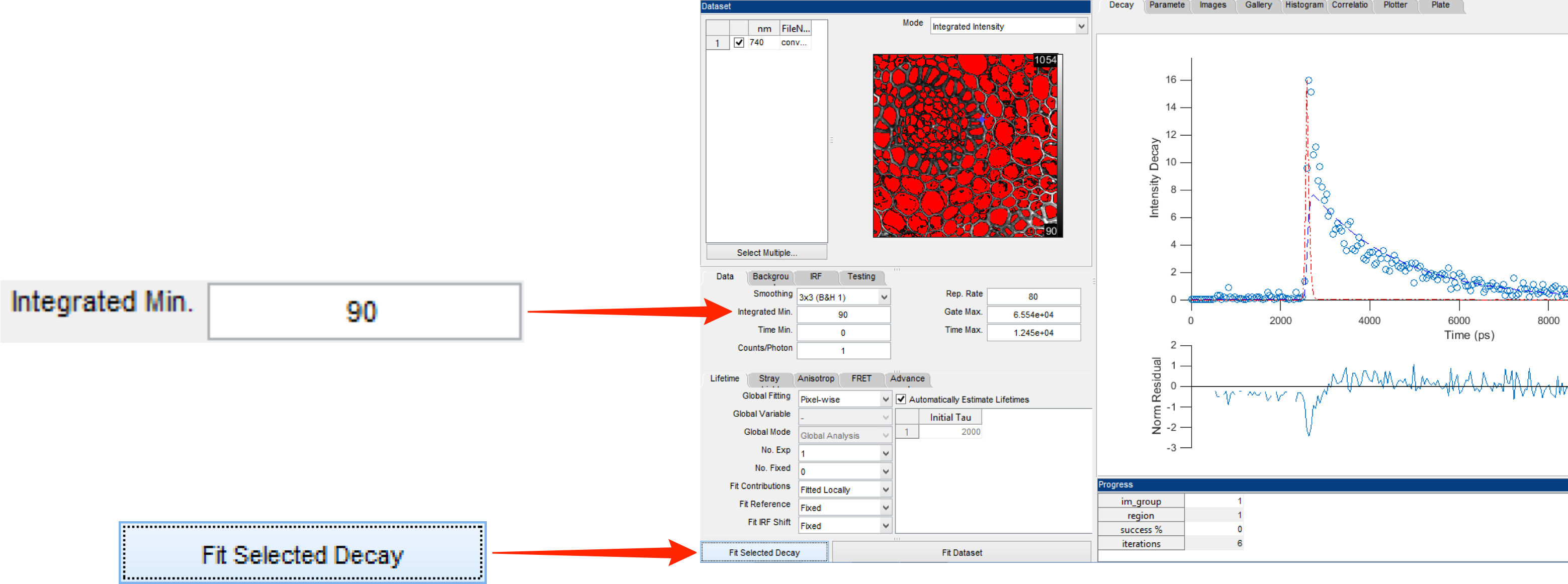
6. By eye, the fit resulting from the default, single exponential, setting does not provide a good fit to this data.

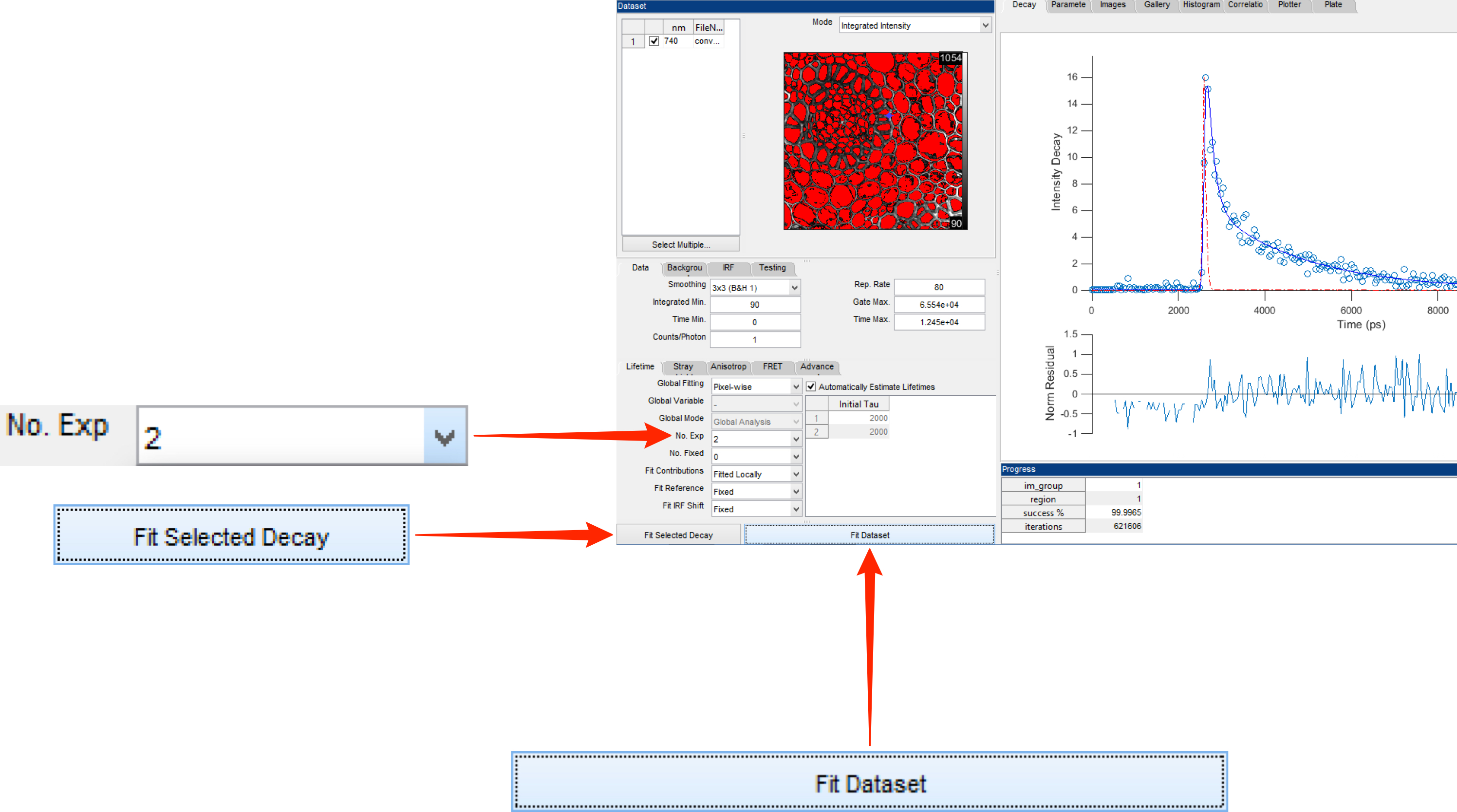
   To try a bi-exponential fit, increase the No Expo to 2 and click Fit Selected Decay.

   The fit of the broken blue line should then look acceptable.

   Confirm this by selecting a few different pixels.

   When confirmed, click Fit Dataset.

   The blue line becomes solid when the dataset has been fitted.

   
   
   
   
   
   
   

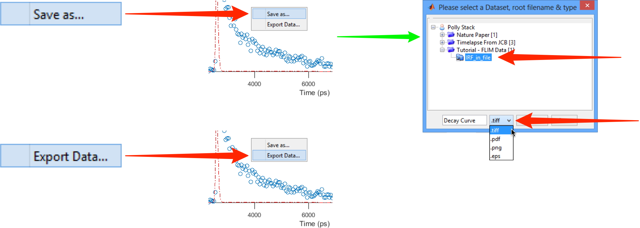
7. The decay plot can be saved as an image, and the data as a CSV file.

   When connected to OMERO the image can be saved to the OMERO server.

   Right-click on the plot, select Save as....

   Select the destination dataset in the data tree and image format from the drop-down.

   Click Save to save the image on the OMERO server.

   If not connected to OMERO, right-click and Save as... will save to disk.

   Right-click and select Export Data... to save the data as a CSV file to disk.

   Use OMERO to upload the file as an attachment.

   
   
   
   
   

Viewing Results

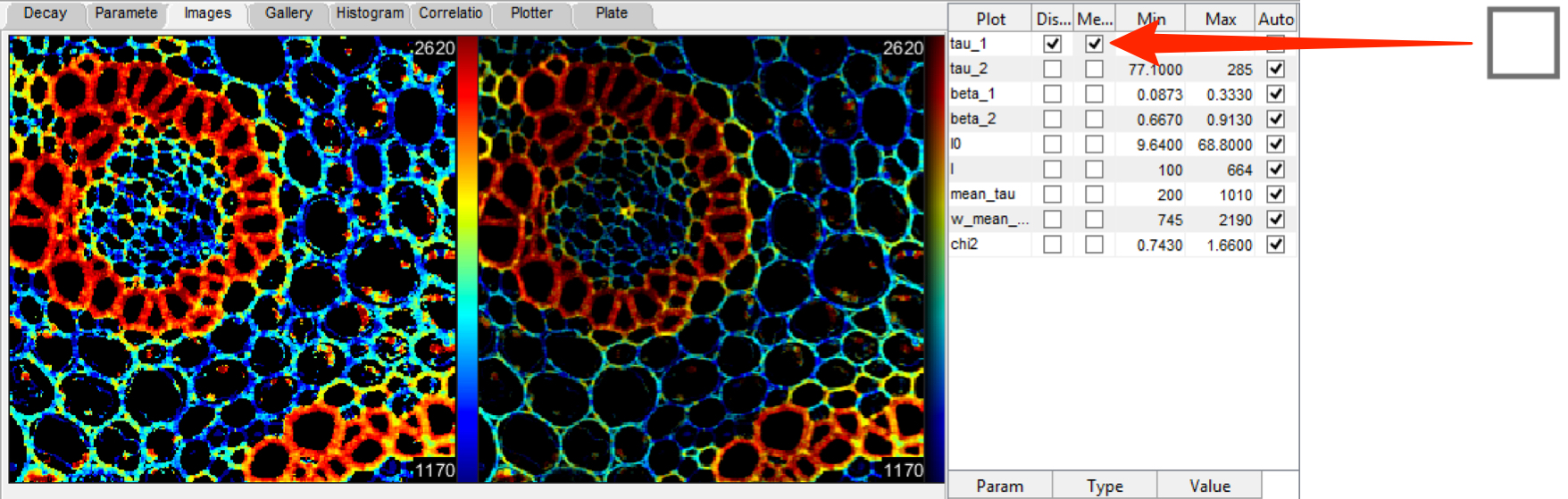
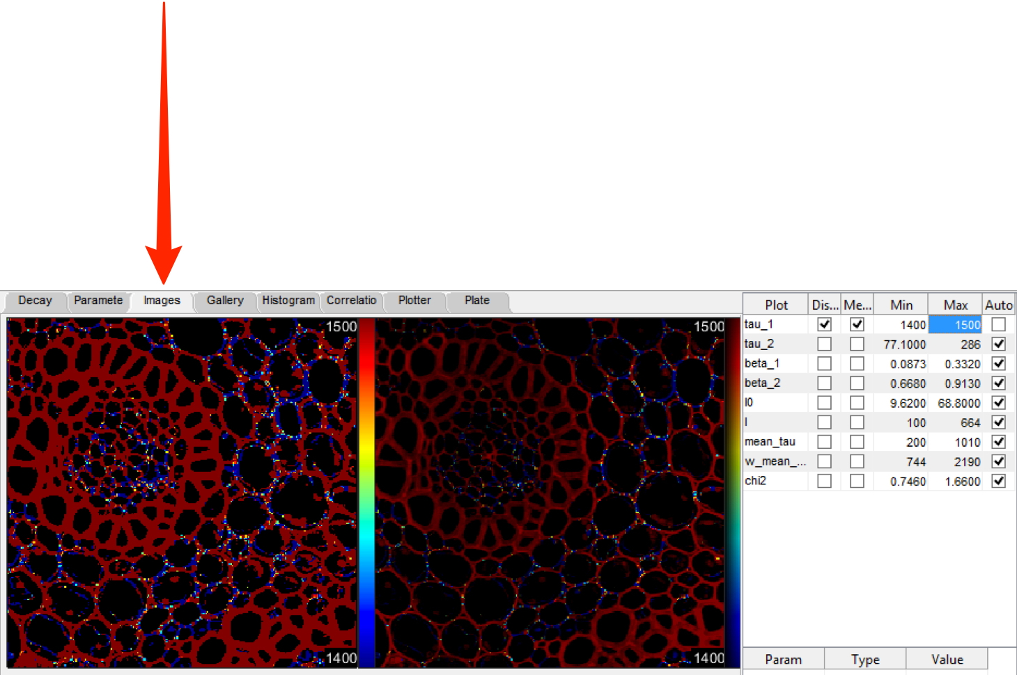
1. When the Fit Dataset processing is complete, select the Images tab.

   At the top right, check the box in the first column of the tau_1 row.

   A false-colour image will be displayed showing the fitted parameter, in this example one of the lifetimes, encoded as the colour at each pixel, along with a scale bar.

   
   
   
   
   

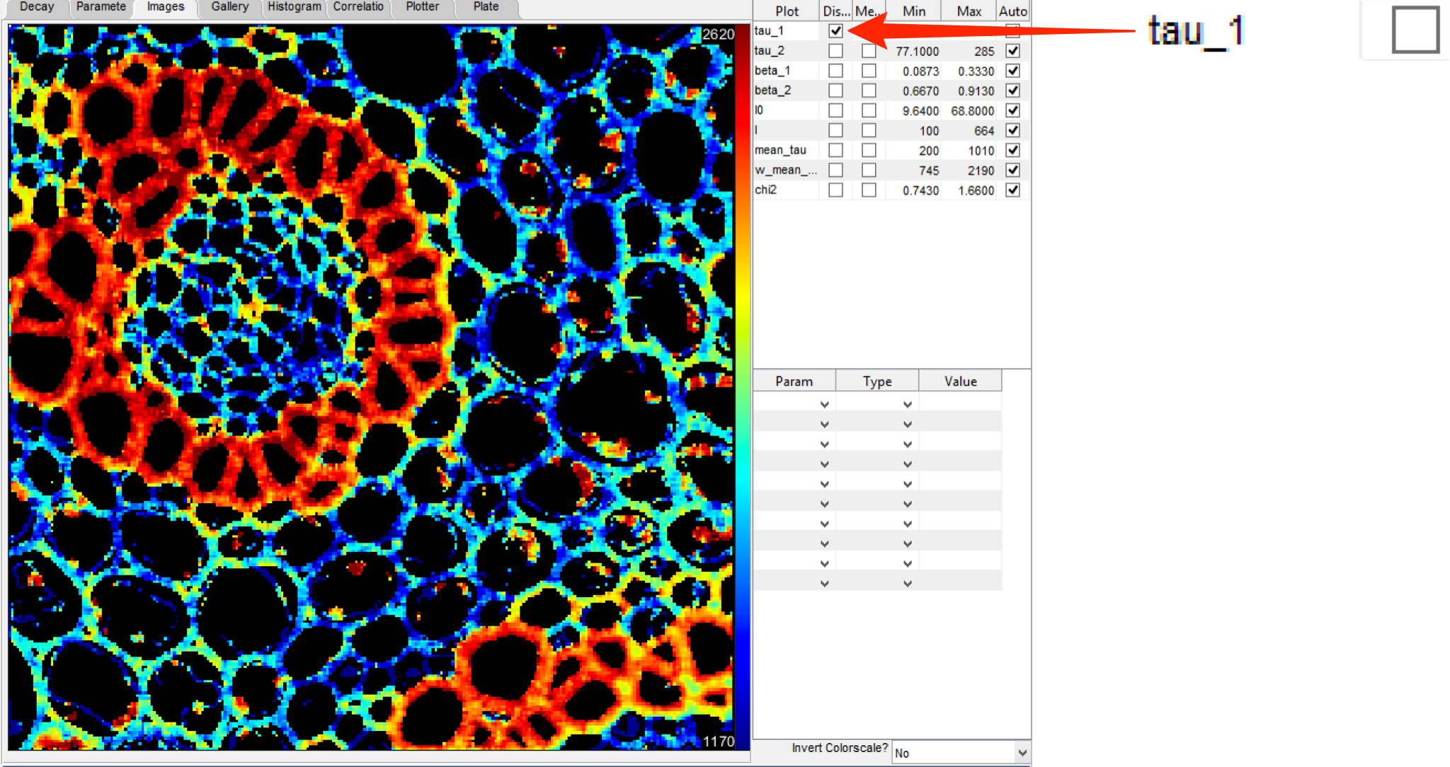
2. Check the box in the second column of the tau_1 row.

   A second image is displayed using the same false colour map but weighted (in greyscale) according to the total intensity at that pixel.

   This de-emphasises the dimmer, i.e. noisier, pixels and displays the structural information in the intensity image alongside the lifetime information.

   
   
   
   
   








3. Select the Histogram tab.

   In the Parameter drop-down, select tau_1.

   
   
   
   
   

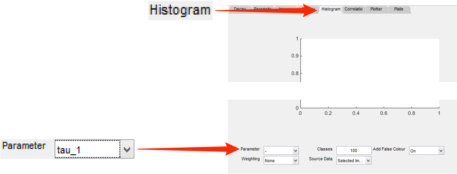
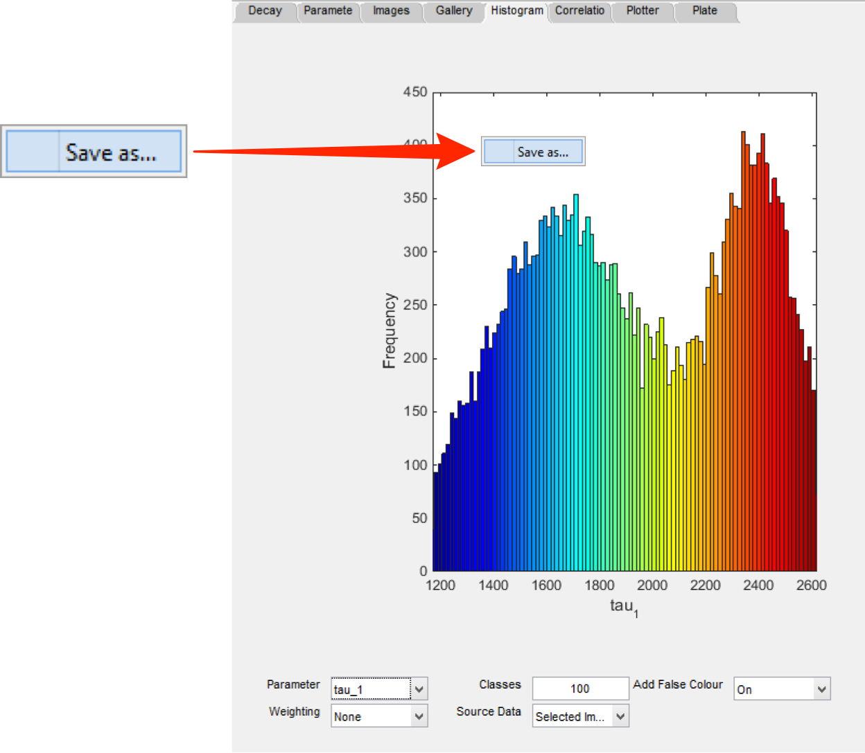
4. The histogram of the fitted parameter has bars coloured to match the display in the Images tab.

   Right-click on the white background of the histogram and select Save as... to save the histogram as an image.

   When connected to OMERO this can be saved to the OMERO server.

   Select the destination dataset in the data tree and image format from the drop-down.

   Click Save.

   If not connected to OMERO, right-click and Save as... will save to disk.

   
   
   
   
   








5. Uncheck the Auto checkbox in the right-hand column of the tau_1 row.

   This enables manual control of the range of lifetimes over which the colour map is stretched.

   Adjust the values in the Min and Max columns to observe the effect on the histogram.

   This allows emphasis of chosen features e.g. a small change in lifetime in a chosen part of the image.

   
   
   
   
   

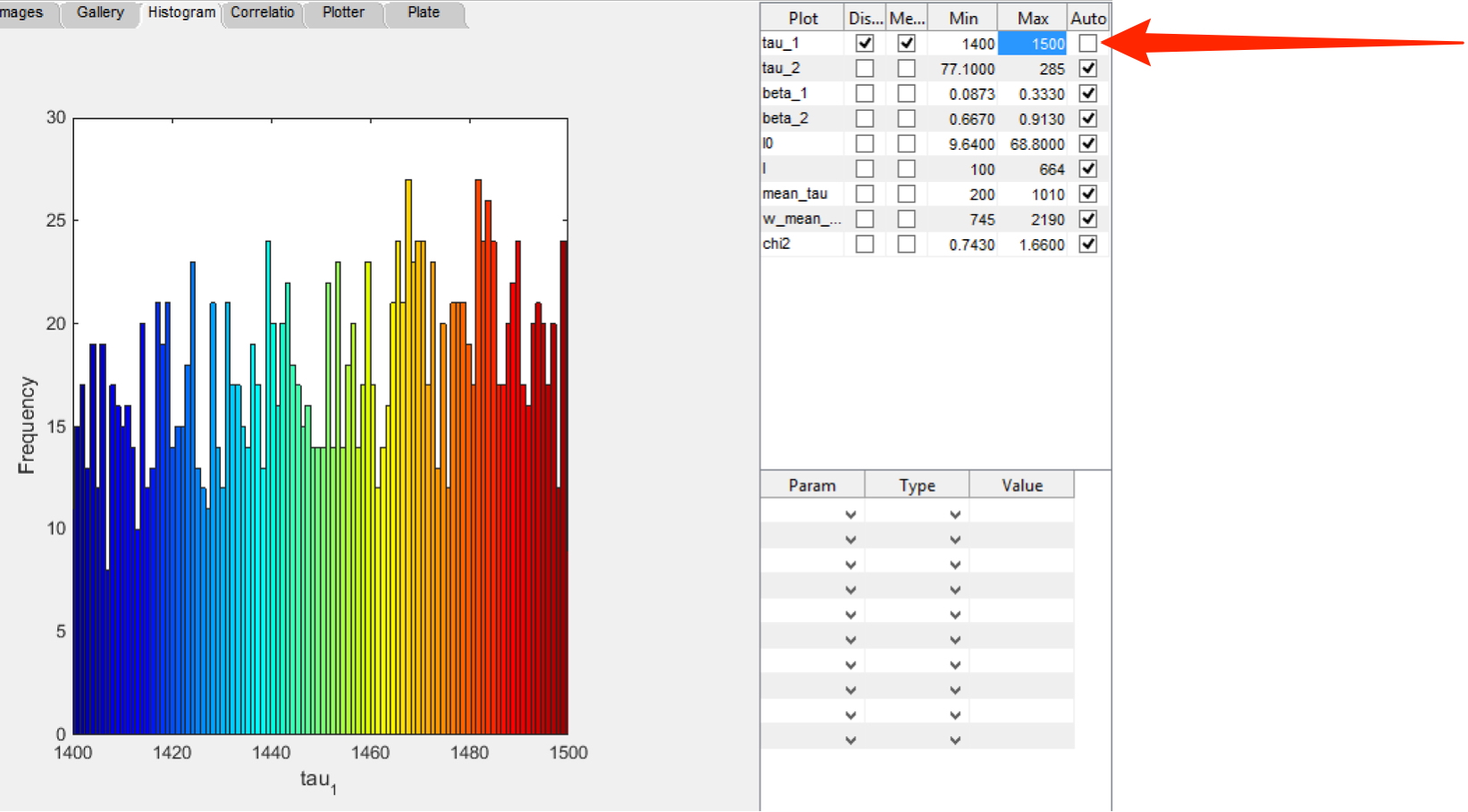
6. Click on the Images tab to see the changes.

   
   
   
   
   








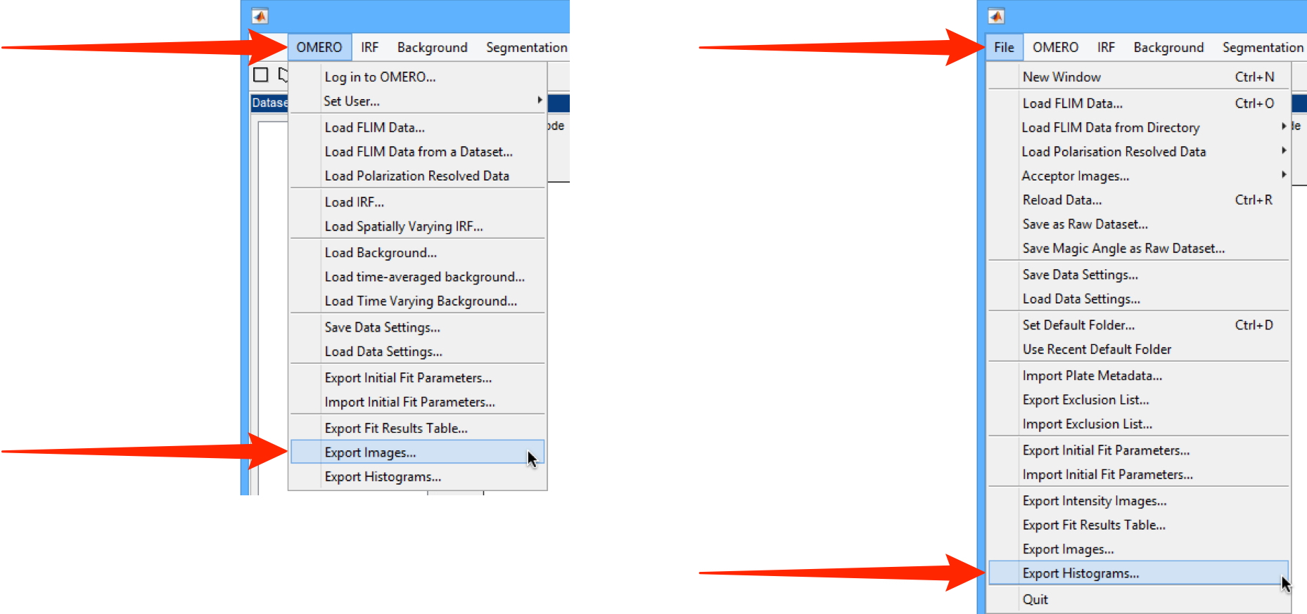
7. From the OMERO menu, select Export Images... to save selected images to OMERO.

   From the File menu, select Export Images... to save selected images to disk.

   Select Export Histograms... to save the histogram data to disk as a CSV file.

   
   
   
   
   

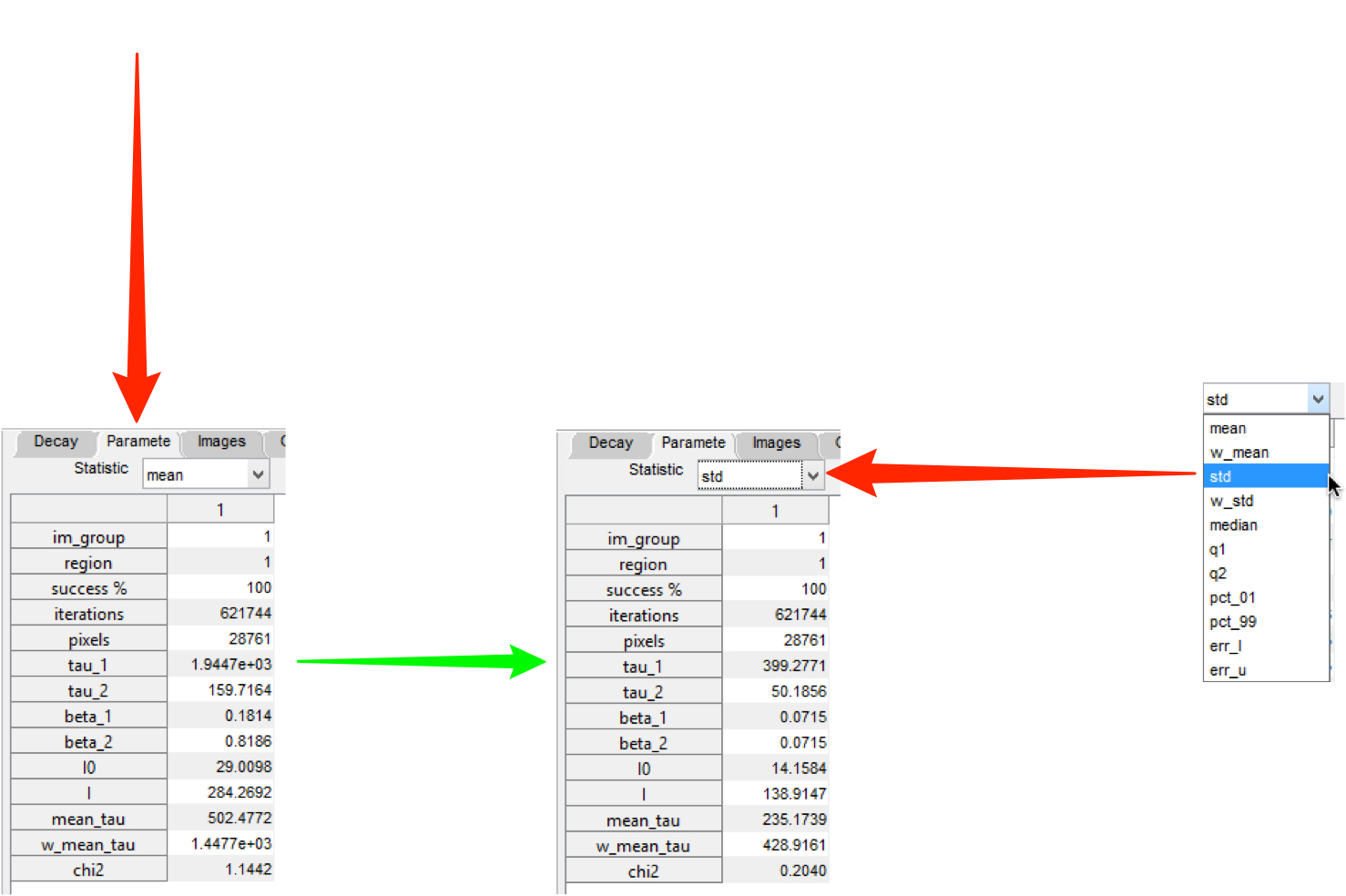
8. Select the Parameters tab to see a table of the mean values of all the fitted parameters.

   Using the Statistic drop-down, select Std to display the Standard Deviations.

   
   
   
   
   

Fitting data - multiple images

Using OMERO, attach the IRF 2013-05-22-T-15-36-21.irf file from the Multiple folder in the downloaded data example to the Multiple dataset created earlier.

See Managing Data for details on attaching files.

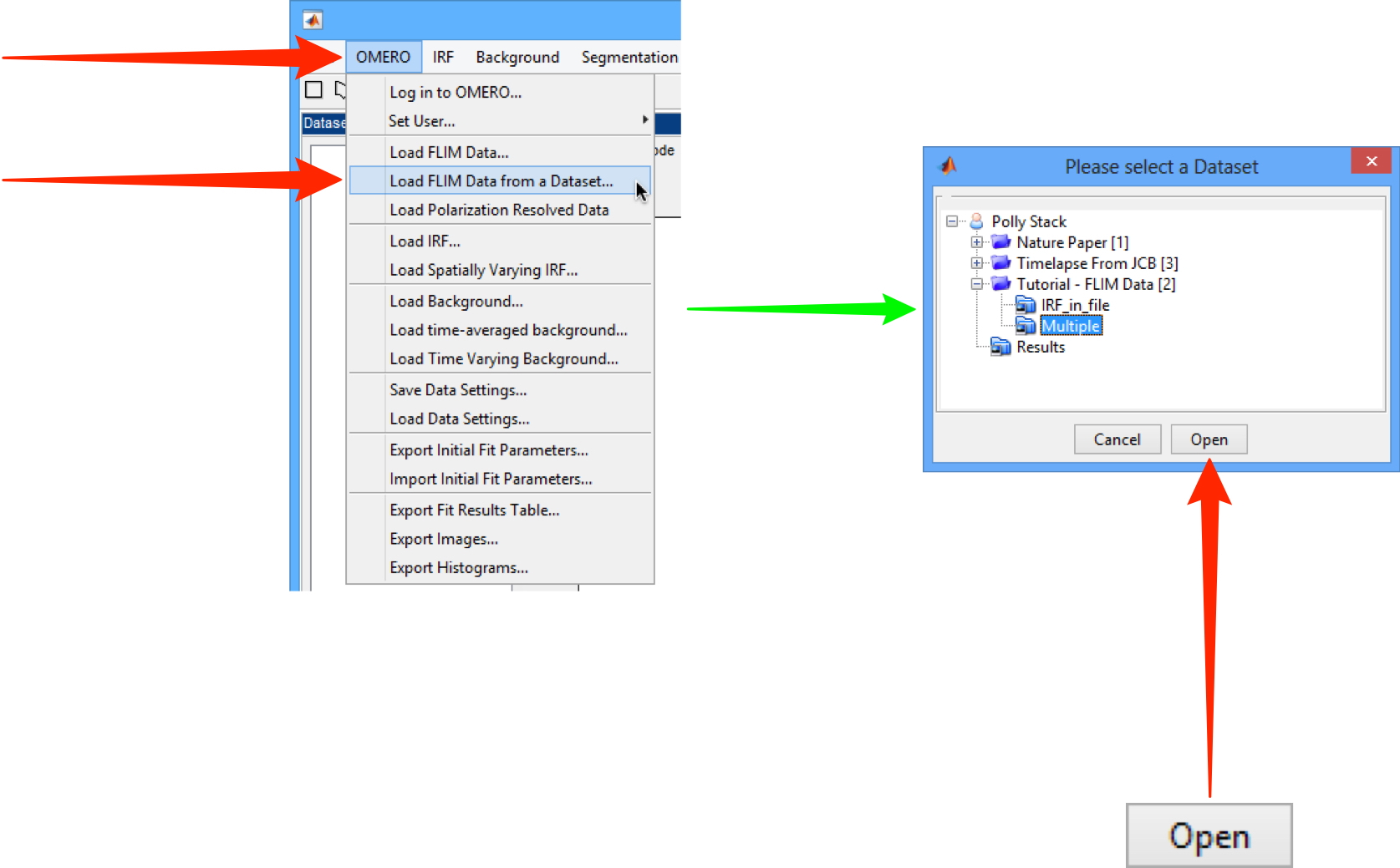
1. Back in FLIMfit, click on the OMERO menu and select Load FLIM data from a dataset.

   The OMERO data tree will be displayed in a pop-up window.

   Select the Multiple dataset and click Open.

   
   
   
   
   

2. Each file in this data contains two separate images, indicated by the suffixes ending in [...#1] and [...#2].

   For this example only the first image of each pair should be loaded.

   Enter 2] into the Filter by name field.

   Click Deselect.

   
   
   
   
   






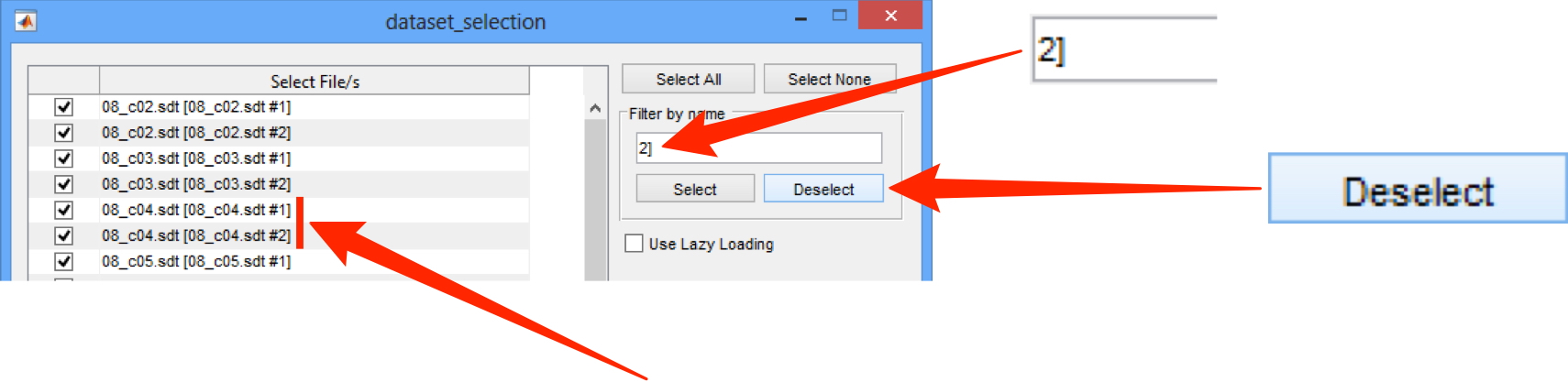
3. This leaves just the images with the [...#1] suffix selected.

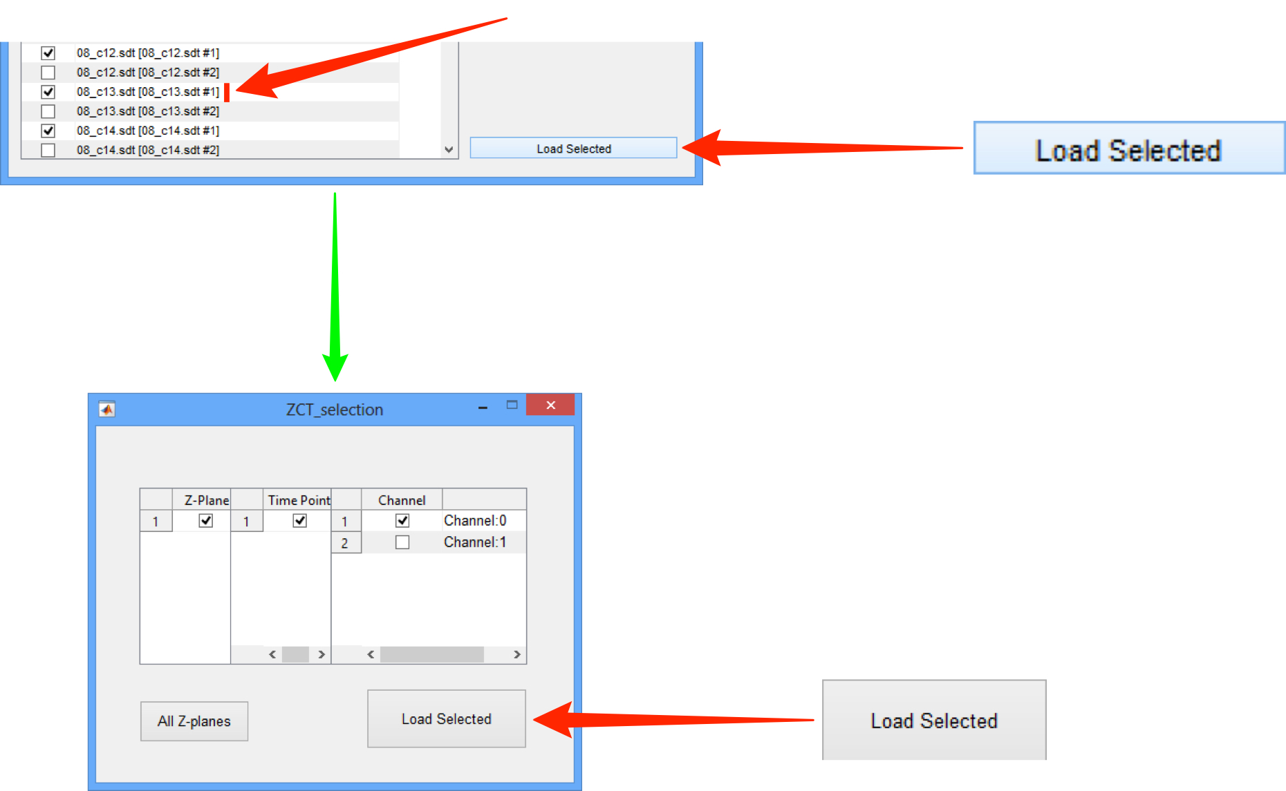
   Click Load Selected.

   The ZCT_selection window shows the data being loaded is 2-channel.

   Channel:0 is selected by default.

   Click Load Selected in this window.

   
   
   
   
   






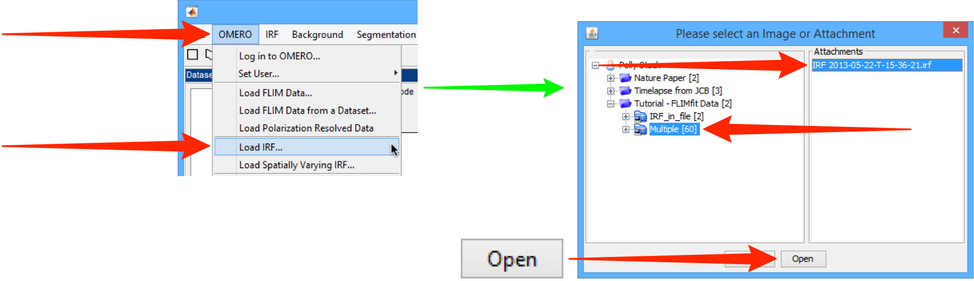
4. To load the IRF for the multiple files from the attachment on the dataset, select the OMERO menu and choose Load IRF ....

   In the left-hand pane of the window, select the folder:        Multiple.

   In the right-hand pane select the attachment:        IRF 2013-05-22-T-15-36-21.irf.

   Click Open.

   The IRF data will be visible as a red peak on the plot in the Decay tab.

   
   
   
   
   



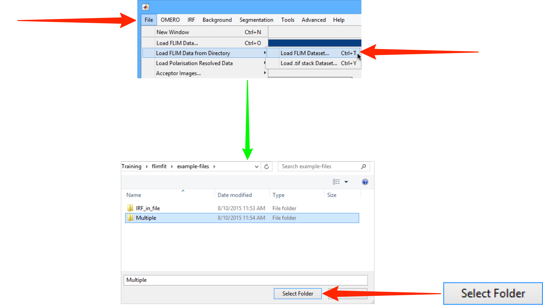
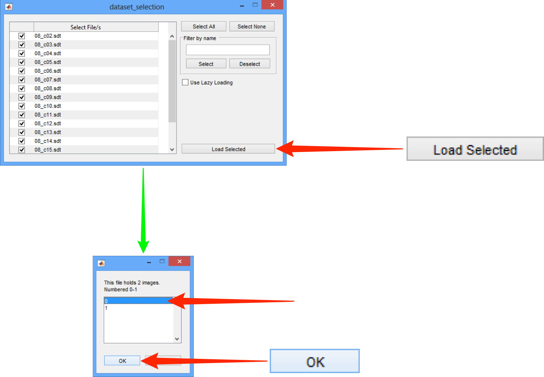
5. To load the multiple file data from local disk, click on the File menu and select Load FLIM Dataset in both levels of the menu.

   In the file chooser select the folder:        Multiple.

   Click Select Folder.

   
   
   
   
   








6. In the dataset selection window, click Load Selected.

   In the following window select the 0 set of images.

   Click OK.

   
   
   
   
   



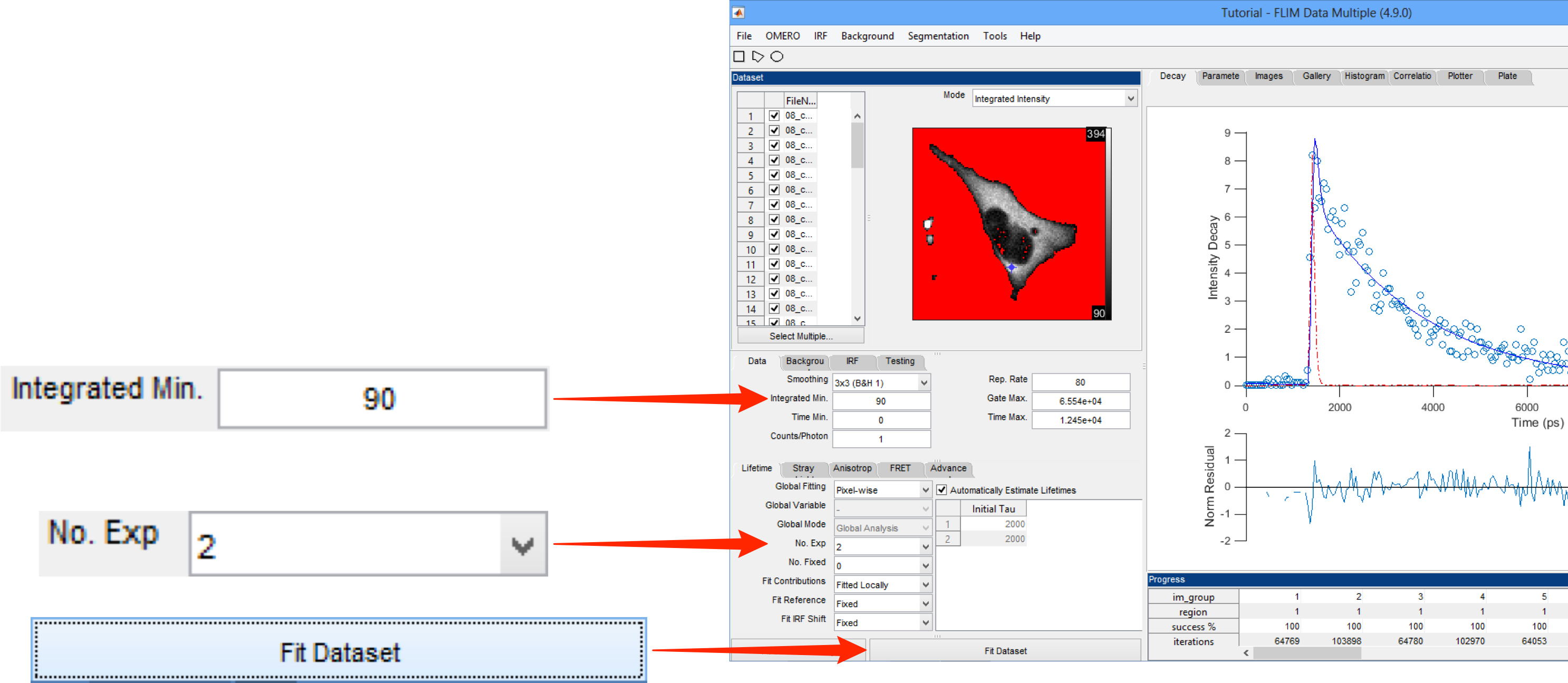
7. Set the Integrated Min to 90 to exclude the dark areas of the image.

   Select 2 in the No Expo drop-down.

   Click Fit Dataset.

   Normalised Residuals are displayed below data.

   
   
   
   
   








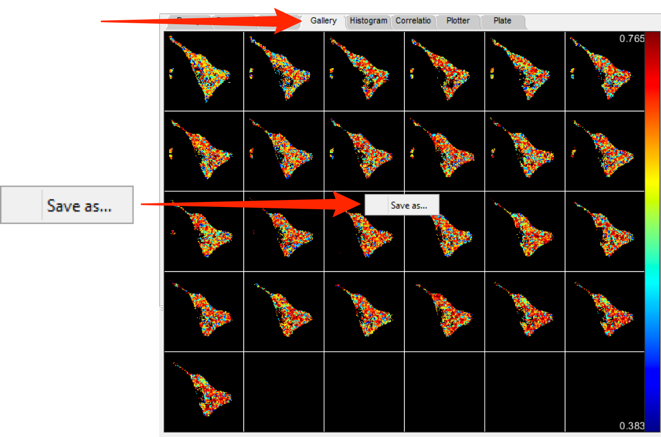
8. Select the Gallery tab when fitting is complete.

   Select mean_tau from the Image drop-down at the bottom left of the Gallery tab.

   Right-click on the gallery and select Save as... save the gallery as an image to OMERO.

   
   
   
   
   

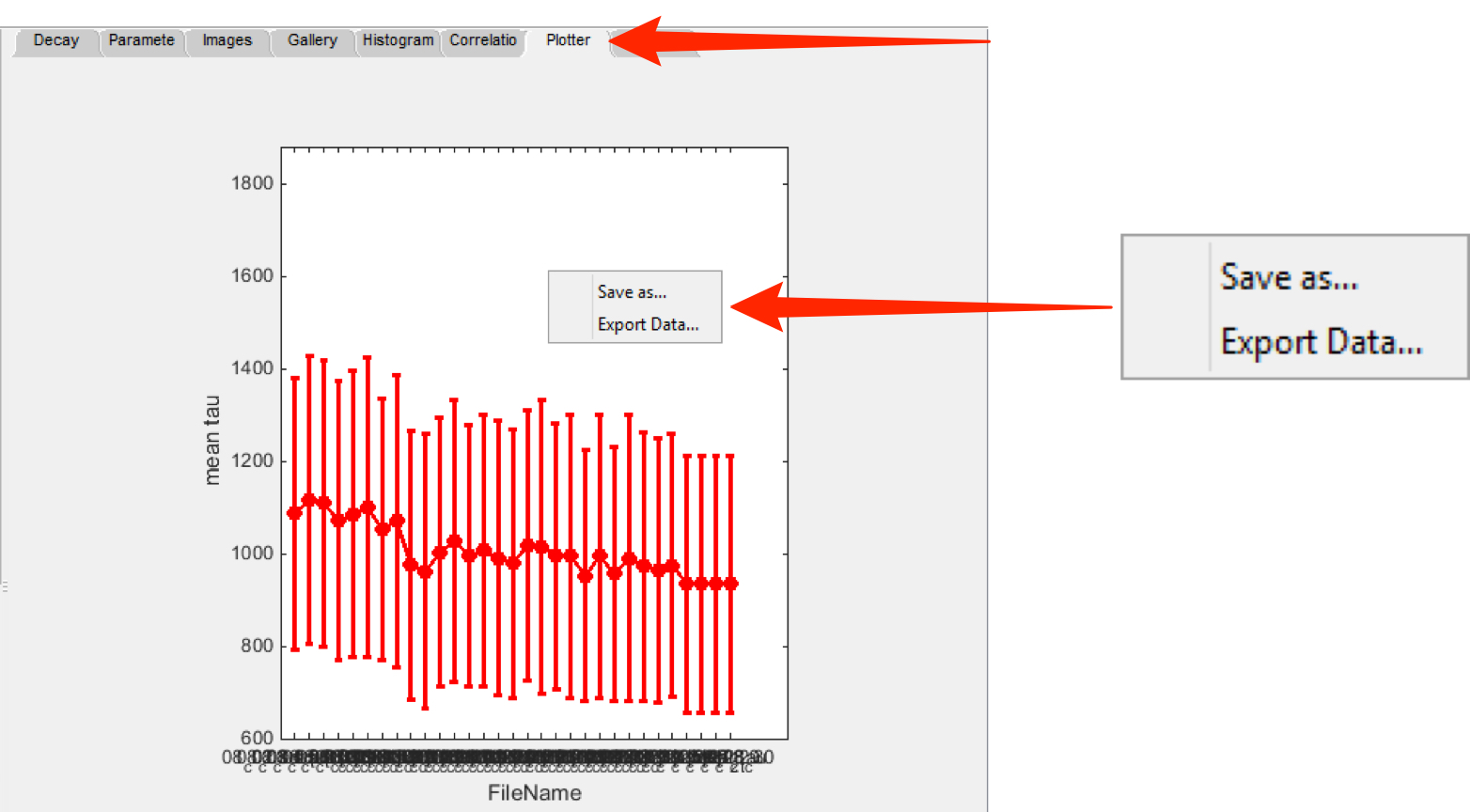
9. Select the Plotter tab.

   Select mean_tau from the Parameter drop-down at the bottom left of the Plotter tab.

   Right-click on the plot and select Save as... save as an image to OMERO.

   Select Export Data... to save the plot data as CSV file.

   
   
   
   
   

Other OMERO interactions

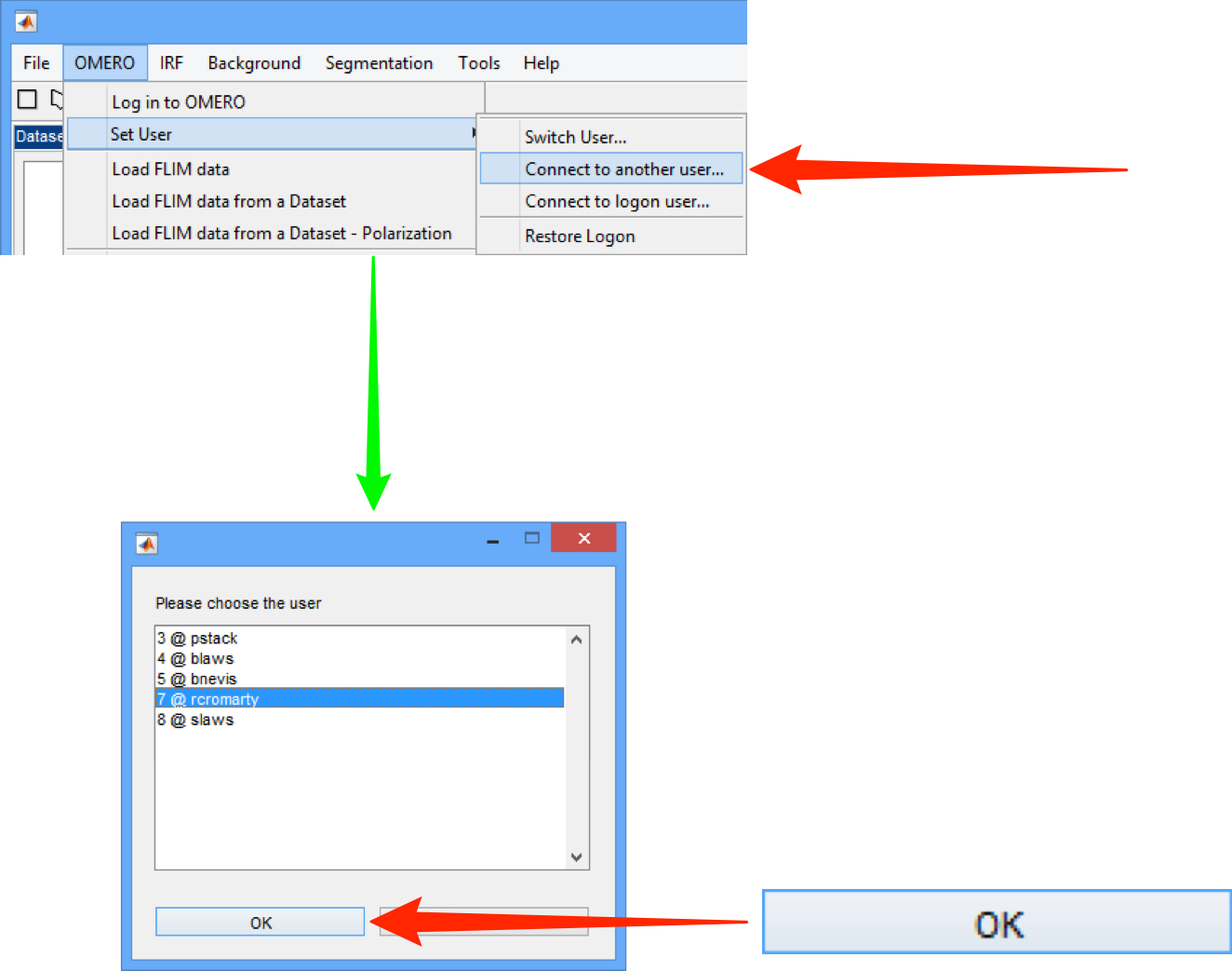
Changing OMERO user

1. To load data owned by another user in your OMERO group select the OMERO menu.

   Navigate to Set User....

   In the dialog, select the user whose data you wish to load.

   Click OK.

   When loading data you will now see this user’s data tree to select data from.

   Use the same process to return to selecting from your own data.

   
   
   
   
   






Other available functionality

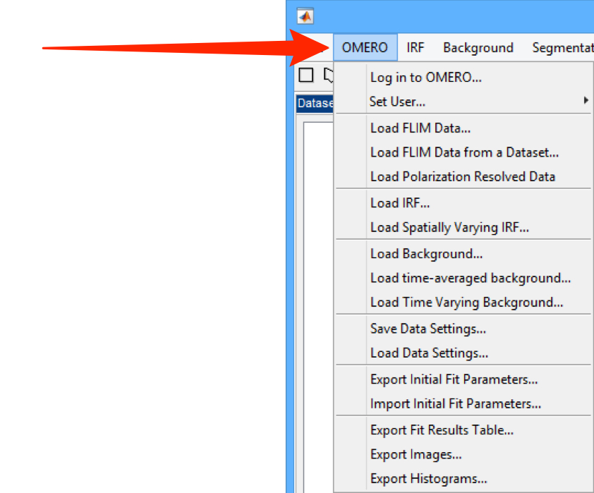
2. The OMERO menu offers a number of other options for working with data from OMERO, and saving data and results back to the server.

   
   
   
   
   

Working with local data and disks

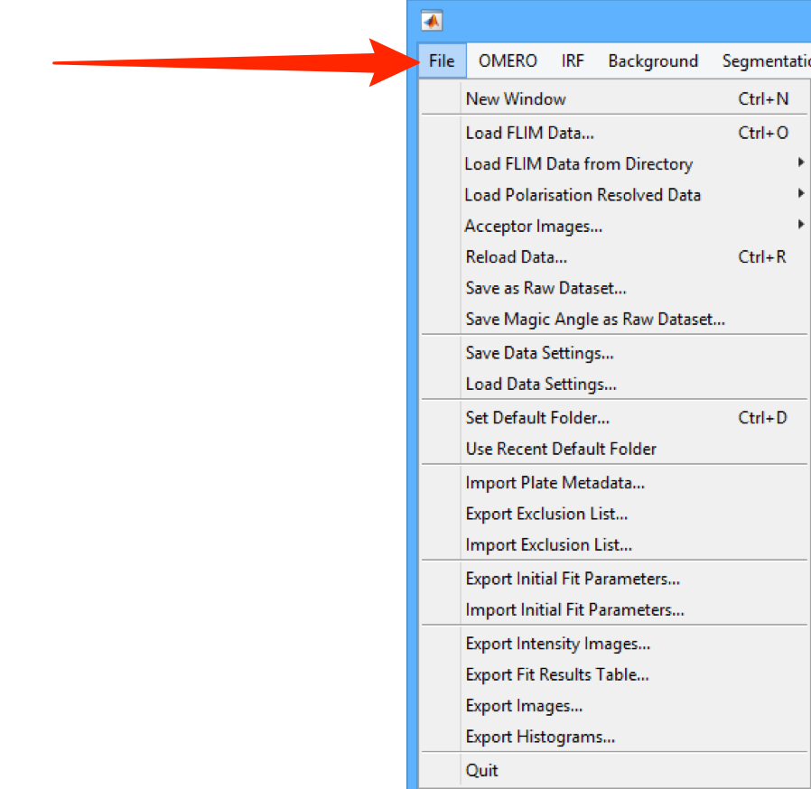
3. The File menu offers all the load, save and export functionality for using data without connecting to OMERO, and for saving results and images back to local disks.